by Michael Delany
With download included in conclusion
Introduction
There are many software packages that can be used for plotting the transfer function of an electrical system. Mathematica is one that’s been around for quite some time and has a very rich set of tools available to it. It is convenient to also vary certain parameters on-the-fly and view the response when doing so. This segment will detail a simple circuit and how to vary key parameters and view the frequency response and output due to the unit step input.
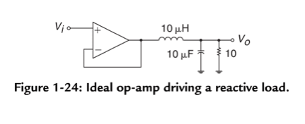
The following is a figure from Robert Pease’s text Analog Electronics. As seen in the figure label, this circuit is an ideal op-amp driving a reactive load. This segment will show how to model this circuit in Mathematica, and in addition, show how to use Mathematica’s Manipulate[ ] function to view changes to the damping ratio and the response time of this circuit.
Getting Started
The following line of code demonstrates how to model the circuit as a transfer function:
Note: to use the Greek alphabet, press the esc key followed by the corresponding key (ex. t for tau and z for zeta) and then esc again.
The above code is a modified version of the standard form for a second-order system. The variables τ and ζ can be used to compute circuit parameters, but in the meantime using this notation helps us better understand the behavior of the circuit. Using basic circuit analysis and replacing the circuit elements with variables, one can see that the actual transfer function is:
It can be seen how the variables τ and ζ map to the circuit parameters L, R, and C. By inspection we can see:
τ =

and
ζ =

Categorizing Response
One way to design the circuit is to first look at the type of frequency response that one would desire. One of the important parameters to design against is the damping coefficient ζ. The following are values of ζ and how they are catagorized against a unit step:
0 < ζ < 1: Underdamped
ζ = 1: Critically damped
ζ > 1: Overdamped
Let’s assume for this example we want an underdamped system. This could potentially give a quick response with some overshoot given correct design parameters. As a general rule of thum, ζ < 0.4 will result in excessive overshoot while ζ > 0.8 will result in a sluggish response. Let’s choose ζ = 0.5 and choose the response time τ = 0.00075.
Given all of these factors, let’s look at the frequency response of the system:
The plot above is a Bode plot of the gain and phase of the system. It should be noted that there are two parameters we can vary in this module, namely the response time τ and damping coefficient ζ.
To generate the plot, we use the Bode plot function with the following syntax:
where ω is the frequency in rad/s over the interval
 to
to
 and expr is the transfer function. In the plot above, the BodePlot[ ] function is wrapped by the Manipulate[ ] function so we can vary the parameters τ and ζ.
Response
Before we continue with the Mathematica implementation, let’s determine that the system gives the anticipated response to the unit step. Using the fact that the Laplace transform of the unit step is 1 / s, we can compute the response by multiplying 1 / s by the transfer function. We can see that the output overshoots the target by approximately 0.17 volts
This response also is wrapped with the Manipulate[ ] function like in the first example. You can toy with the response time and damping ratio to see how the response will vary in the time domain.
We can then compute the ratios of the different circuit elements if we know our damping ratio and response time.
Using the Manipulate[ ] function
The manipulate function is quite simple. The user specifies the variables he or she would like to change on-the-fly as an argument to the function.
In the code above, the following syntax is used:
You can see that the same arguments are repeated for the damping coefficient ζ. Again, here is the code for comparison:
Conclusion
We can see that Mathematica is a very powerful computational engine that can be used for many things specific to EEs. Whether it's active filter design or classical control theory, Mathematica will have predefined functions available for you to get your engineering work done. Also, this webpage was generated with Mathematica.
The file used to generate this webpage is also available for download.
Download:
Sources
1. “Bode, Nyquist, and Nichols Diagrams of Second-Order Systems” from the Wolfram Demonstrations Project
http://demonstrations.wolfram.com/BodeNyquistAndNicholsDiagramsOfSecondOrderSystems
2. Ogata, Katsuhiko. “Transient and Steady-State Response Analyses.” Modern Control Engineering. No ed. Vol. 5th Edition. Englewood Cliffs, N.J.: Prentice-Hall, 1970. 159-171. Print.
3. Pease, Robert. “Review of Feedback Systems.” Analog Electronics. No ed. Burlington, MA: Newnes, 2008. 22. Print.


No comments:
Post a Comment